
The Hidden Assumptions of Process Modeling
Deploying a Model with High Confidence as to Which Variables Are Critical Process Parameters (CPPS)
Process manufacturing data is complex. The time series aspect of this data creates challenges. From differences in data sampling rates to inconsistent or custom units to data storage across multiple systems, process data can be difficult enough just to collate and align for modeling. While our engineering training drills into our head that we should always document our assumptions, we often focus solely on the assumptions of the model itself, such as what regression method we used, what training data set we used, or how the model only applies within a certain range of input values. We often overlook some of the key assumptions that went into the data preparation. These assumptions can be critical in deploying a model with high confidence as to which variables are critical process parameters (CPPs) versus a model with just a decent representation of the data set or moderate r-squared value.
First, let’s talk briefly about modeling. Modeling relates to a wide variety of techniques from simple methods such as various types of regression or clustering algorithms all the way to machine learning or artificial intelligence models such as artificial neural networks or random forest decision trees. Regardless of what type of model is chosen, all of these have a vital data preparation step that is rarely examined critically.
Assumption #1: Data Sampling/Gridding
In order to run a model, the data first needs to be aligned. In data science, this is often termed gridding, where the data is resampled at a particular frequency in order to select the closest or interpolated value for each process signal at that point in time. While the gridding period is often selected based on the length of the training window and the amount of computational time it may take to process a certain number of samples, the gridding period is rarely tracked back to the raw data itself. In addition, I have found it uncommon that models will be tested on multiple gridding frequencies to see how the gridding impacts the model.
Let’s take a look at how gridding can drastically impact your data set that goes into the model. In the below picture, I have taken a process data signal of temperature (purple) and gridded that data set at 2 minutes (green) and 5 minutes (red). While the purple signal consists of a distinct oscillatory pattern that represents many process signals, the selected gridding period may completely remove that oscillation as shown with the 5-minute gridding. This inherent filtering of the data may result in the removal of noise in the model, a positive result, or completely miss the critical variable that you were using the model to find.
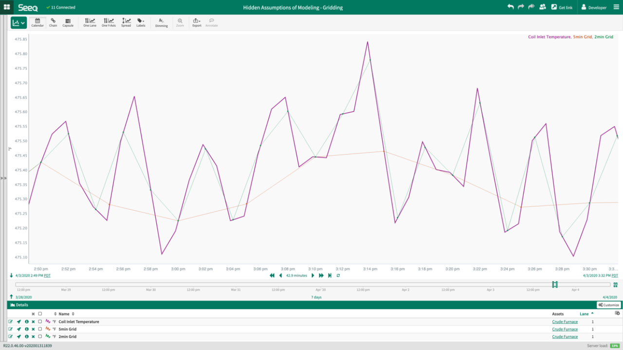
If gridding is an issue, why don’t we just use every data point? There are a couple issues with that approach as well. In addition to the extra computational power required and the high possibility of overfitting models, process data sensors are not sampled at the same frequency or time. Therefore, there will always be some signal that is being filtered unless the most frequent signal is selected as the gridding period. In this case, all process variability will be captured in the data set, but now you must question the validity of the interpolation type, especially if the sampling frequency for inputs to the model differ significantly. By default, data historians tend to interpolate between stored data points, typically using a linear slope between samples. When many interpolated data points are being used in the model, you should question whether that linear slope accurately represents the data or whether some other function, like a filtering algorithm, would better represent the data.
As an added layer of complexity, many historians utilize a notion of compression in order to minimize the size of stored data. With compression, the data is stored at an inconsistent rate, where a new data point is created only when a specific deviation in value is observed or if a maximum duration has been exceeded. This results in inconsistent data sampling frequencies. If original timestamps are used as the gridding for the model, the model is effectively weighted to favor periods where data variability was greater due to the presence of more sample points.
The takeaway here is that there is no precise workaround for selecting the perfect gridding period. You should always document the assumptions you are making during the gridding process and understand the differences between the gridded and actual process data, preferably by visually comparing the gridded data set against the raw data. Checking for differences with multiple gridding periods or including additional information into the model (e.g. moving window standard deviation to capture oscillations) are some ways to verify that gridding did not impact your model results. This also stresses the impact of having access to the raw data source. If you had to ask for an export of the data and it comes back with aligned timestamps and a consistent sampling period, the data has most likely already been gridded and is not the raw data as it exists in the historian.
Assumption #2: Aligning Data by Time
One of the most common mistakes I see in data preparation is the default position of aggregating data by timestamp. While it may make sense to compare multiple signals based on an equivalent timestamp, there is an intrinsic assumption built into that comparison that the process fluctuations at the exact same time across all sensors. However, the best way to align data is usually by material flow. For example, if we want to know which process variables impact the quality of a particular product, we would want to know when the slug of material that has a quality measurement was measured by each sensor upstream in the process. In a short, rapid process, the difference between aggregating by time and material slug may be negligible. On the other hand, a long process may have hours of delay between sensors and the quality parameter.
As an extreme example, let’s think about a pipeline – whether it is transporting oil, water, some other material, or even is a plug flow reactor. Some pipelines may be miles (or 1,000s of miles) long with various sensors throughout measuring fluid characteristics like temperature and pressure. The quality of the material may be measured at the end of the pipeline, which could have taken minutes, hours, or even days to arrive. If you want to know what additives, temperatures, or other variables influenced the quality of that product, you would want to track that material back through the pipe and determine the signal values when that material passed each sensor; for example, the additive flow rate that was present when this material passed the flow meter or the temperature of the material when it passed the temperature probe rather than taking the active measurements at the end timestamp.
Most processes fall somewhere in between these two extremes where the data requires some shifting of time to improve the understanding and applicability of the underlying model. The ideal time shift for data is often what is known as the residence time between sensors, which can be calculated by the volume of the system between each sensor divided by the flow rate of the system. As the flow rate fluctuates throughout the process, this time shift is not a constant time unit, but a variable time that will fluctuate based on how fast the system is processing.
Assumption #3: The Data is Representative - Missing the Trajectory
Batch processes avoid many of the time shift requirements in the previous assumption but come with challenges of their own. During batch processes, the process is often in a transient state. While some online quality measurements exist, many offline quality measurements still persist where samples are taken periodically throughout the batch to check for relevant quality criteria. These batch samples are generally discrete measurements and only a few samples may be taken per batch, either requiring interpolation between data points or significantly limiting the data set for modeling.
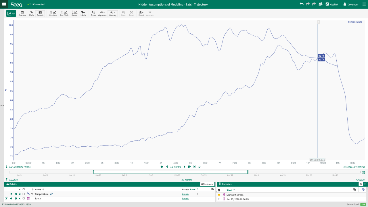
Batch processes have an additional complication the data point at a particular timestamp is not the important part, but the entire trajectory of the batch up to that point in time. For example, I have two overlaid batches in the figure below. If the quality sample measurement was taken at the time of the cursor (approximately 10 hours and 19 minutes into the batch), both process data measurements would be equivalent at that time period at 93°F. If that was the only data that was gridded for the modeling techniques, we would entirely miss the trajectory of the temperatures that the process went through to get to that point. In the case of a reaction, the differences in temperature profiles during the process leading up to that sampling point would likely impact quality and/or yield even though the model data set would assume they are the same input data sets.
It is critical to include some representation of the batch trajectory when modeling a batch process as the quality or yield at any point within the batch is a function of all the batch data up to that sample point. There are a wide variety of options for incorporating these batch trajectories ranging from simple statistics (e.g. totalizing oxygen flow rate to get total oxygen added to a bioreactor) to dynamic modeling methods. In addition, the use of golden profiles or golden batches can help restrict the model to batches that fit a desired trajectory; this is a similar approach to restricting the input parameters of a model to the range of input parameters that was available in the training data set.
Assumption #4: Using Raw Data without Consulting the SME
If I were to have one key take home message from this article, it is that the modeler should always collaborate with the subject matter expert (SME). Data sets are confusing. In addition to all of the previous assumptions discussed, there are a wide host of hidden secrets that only the SME can assist with. The modeler often respects the data as the law and avoids modulations of the data. However, there are times when calculations are required to make the models match physical reality. How many times have you seen a kinetic model fit on degrees Celsius instead of converting to absolute temperature? Or a model using gauge pressure that just doesn’t fit correctly because it wasn’t converted to absolute pressure? The SME likely deals with these issues on a regular basis and should be able to help sort through the necessary data preparations.
Consulting with the SME to fully understand the process can also result in more productive outcomes. Has a model outcome ever been something completely obvious to the SME like that temperature and pressure are inversely related in a gaseous reaction? SMEs provide a wealth of knowledge about the process including known correlations between variables that may result in multicollinearity, variables that should be combined due to the synergistic effects in the process, or constraints on process changes that can be made. For example, a model that tells you the best quality would be achieved if we could increase line speed and decrease tension is pointless if those two variables are intrinsically linked or it is not feasible to adjust these variables.
Data preparation is an important step that is often overlooked in process modeling. Each process is different enough that the modeler should think carefully about the various assumptions that are going into the data preparation process. The appropriate gridding of the data, understanding what the best method is for data alignment, incorporating the trajectory of variables for batch or process run models, and collaborating extensively with the SME are all vital steps in building the best process model to leverage for process optimization and improvements.